Lab5 - Linear PID Distance Control and Linear Extrapolation

Objective

The purpose of this lab is to implement linear position PID control and pick whatever controller works best for the robot system. Use the control system to let the robot drive as fast as possible towards a wall, then stop when it is exactly 1ft (=304mm=1 floor tile in the lab) away from the wall using feedback from the ToF sensor.

Keywords

BLE, PID Control, Extrapolation

Prelab - Optimization of BLE Data Transfer Module

The general idea is similar to lab1 – Use BLE to transmit data between Artemis and our own PC. I implemented this module by first collecting all the related debug data readings (e.g. time, distance readings from ToF, PWM duty cycle value of the left and right motors…), and then use a function/case to continuously transmit all the data in one go. On my PC, I receiving the data by first connecting the Artemis board BLE through the MAC address, and then parsing the transmitted strings by the optimized notification handler.

In my Artemis board code, I implemented the case SEND_DEBUG_READINGS which is used to send the data to the PC. All the array variables were pre-defined as the global variables.

On my PC, the corresponding handler was modified as:

In this way, I can directly access all the wanted debug readings which would be stored in those arrays (e.g. generating the plots of Distance error vs Time).

Lab Tasks

Task1 - ToF Sampling Time Discussion

In this lab, considering the requirements that the robot car should start 2 ~ 4 meters away from the wall and the ToF’s sensing range, I generally chose the long distance mode because the range of short distance mode is [0, 1.3m] with the extreme limit 2m, and the range of long distance is [0, 4m] with extreme limit 4.3m. After I tested the sampling rate of the ToF, I found that the difference bewteen the rate of PID control information updates and the rate of ToF sampling quite big. (The standard sampling rate of ToF is about 50Hz, but in practice is quite slow when there are other constraints, such as the completion of soldering and the code latency)

Based on this performance, it is necessary to implement filters or extrapolation to make the ToF readings “updated” more frequently.

Task2 - Range of P-Controller Gain

Here, we can only implement the PID control in discrete time. For the P-controller, the gain can be calculated as $P = K_p \times \text{Error}$. The range of the PWM value for the function analogWrite() is [0, 255]. Also, during past labs, the motors’ deadband is approximately 65, and the Error can be a thousand. So, based on - $K_p \times \text{Error} + 65 \in [65, 255]$, we can accrodingly get the rough range of the P-gain: 0~0.5.

Task3 - P/I/D Discussion

This task is to deploy the PID control on our robot car. I basically followed the heuristic procedure (#1) to find the value of P/I/D:

Before I implemented the PID, I added another case to initialize all the PID-related parameters:

Also, I set the maximum forward PWM values to 120~150 to make the robot car easier to slow down during experiments.

P-Controller

The general implementation method of P-controller is: $P = K_p \times \text{Error}$.

I first tried the P-controller, setting Kp from 0.001 to 0.5. Then, I found that when Kp was from 0.1 to 0.2, the robot car’s performance was great. I plotted the distance error (dist_error = current_distance - target_distance) and the real-time PWM values as follows when Kp was 0.1:

And the distance error and the PWM values for Kp=0.2 are:

The video for Kp=0.2 is shown as below:

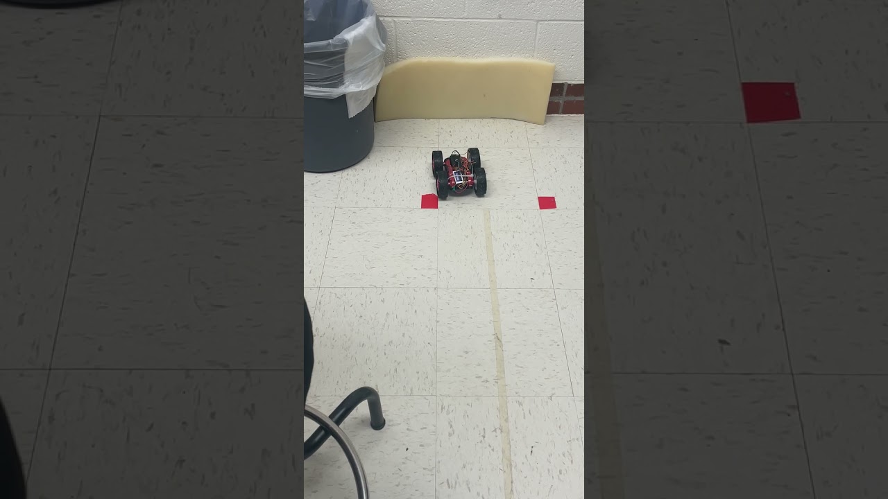
From the above two groups of images, the car could overally complete the lab task. But the overshoot and the rise time were not so great. After many rounds of tests, I finally set the Kp as 0.15 which could stably perform well.

PD-Controller

After I had my P-controller, I began to add the Derivative term to my control module. Bascially, D-controller can be implemented as: $D = K_d \times \frac{\text{DistanceError}^{(t)} - \text{DistanceError}^{(t-1)}}{dt}$

Generally, when I implemented the PD-controller, the distance error’s overshoot became smaller, and the overall curve got better. More importantly, the car’s performance bacame much stabler than that only with P-controller.

The distance error from (Kp, Kd) = (0.015, 0.005), the P/I/D real-time values, and the real-time PWM values are as follows:

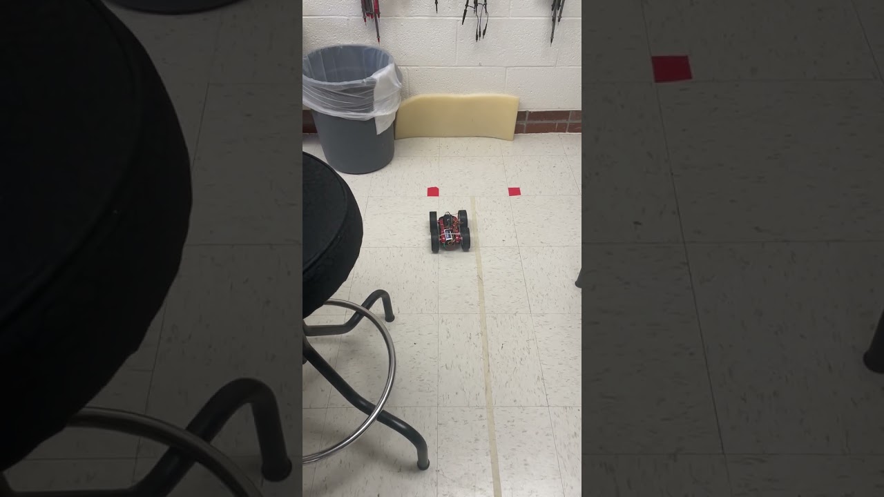
Also, the video for this stage is:

PID-Controller

Finally, I tried the PID-controller. For discrete cases, the integration term can be implemented as: $I = K_i \times ((\sum_{j=1}^{t-1}\text{DistanceError}^{(j)}) + \text{DistanceError}^{(t)} \times dt)$.

The integration term accumulates all the past error terms and reflect it to the general PWM values. So, I set the value clamp to the integration term. The PID controller made the distance error curve smoother and the overshoot became smaller. Also, the status around the target distance was also quite stable.

After rounds of experiments, I set (Kp, Ki, Kd) = (0.15, 0.1, 0.05). The corresponding reading plots are shown as follows:

I took three video clips to show the PID-controller’s stability and performance:

First:

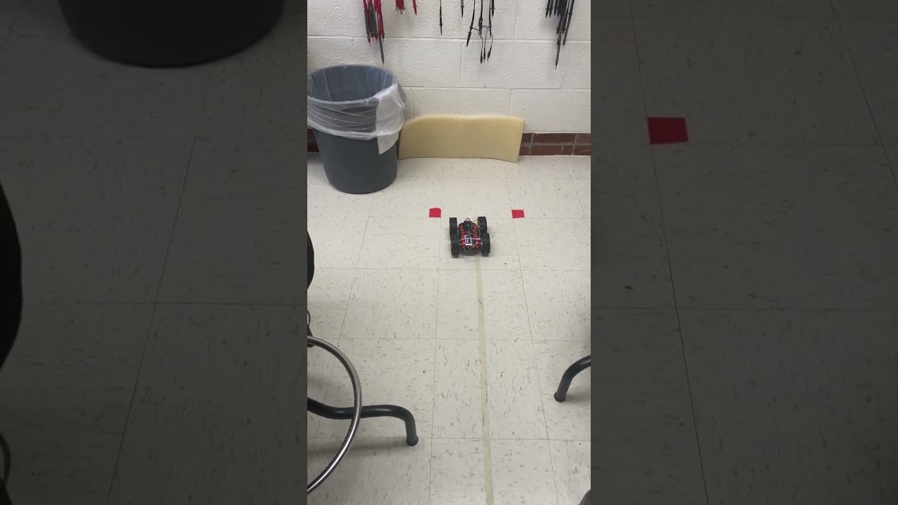
Second:

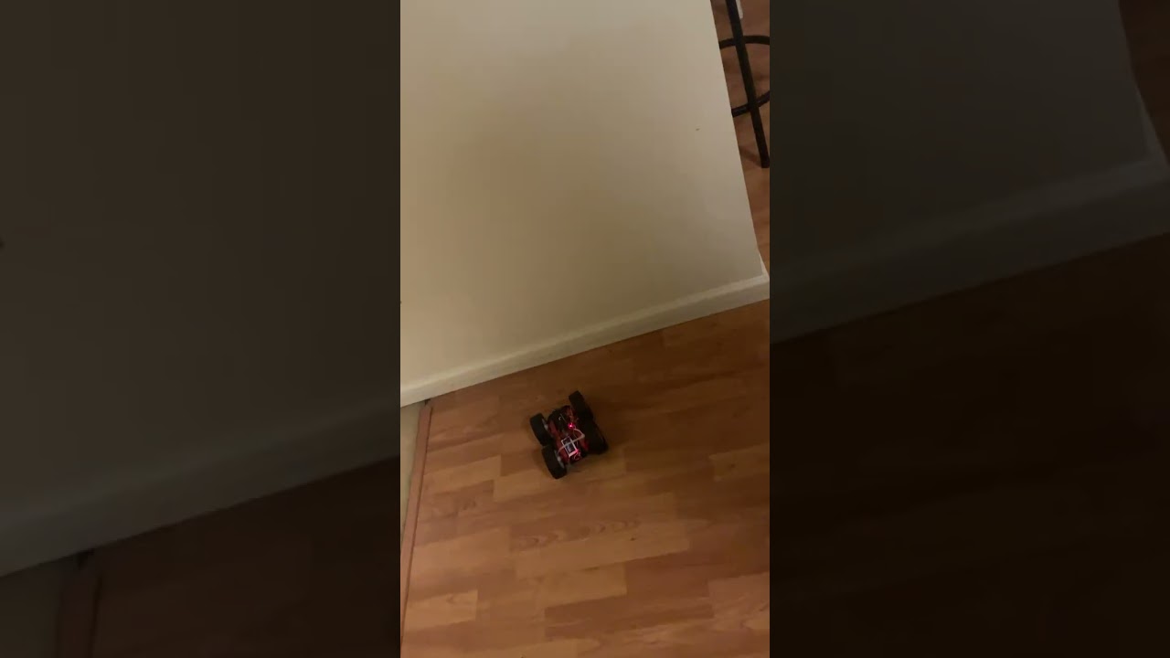
Third:

From all the tests, I found that PID controller can let my car “converge” more quickly and with less time “wandering” around the target distance. However, we can clearly discover that the plots were all “cut” into horizontal pieces due to the different sampling rates between the PID loop update and ToF reading update. I then tried to implement the extrapolation to greatly optimize this problem.

General PID Control Code Block

Here is the general code of PID control implementation:

Notes: The clamp for integration term was set to 50. The general PWM clamp was set to 120.

Extrapolation

Generally, we can implement the extrapolation as: \(\text{PredictDistance} = \text{PrevDistance} + \frac{(\text{Current ToF DistReading}) - (\text{Previous To DistReading})}{(\text{Time Gap between the Last Two ToF Distance Readings})} \times (\text{Time Gap of the Last Two Time Readings from PID Loop})\)

In my PID loop, the code is like:

After testing, the results and performace were really good. The curves and the car’s motion became much smoother.

Without Extrapolation, the readings are like:

With Extrapolation, the readings are:

We can easily discover that the extrapolation can greatly optimize the gaps between each ToF reading updates.