Lab7 - Kalman Filter

Objective

The objective of Lab 7 is to implement a Kalman Filter, which will help to execute the PID-related behaviors in Lab 5 faster. The goal now is to use the Kalman Filter to supplement the slowly sampled ToF values, such that you can speed towards the wall as fast as possible, then either stop 1ft from the wall or turn within 2ft.

Keyword

Kalman Filter

Mathematical Theory Foundation

The Kalman filter provides a systematic way to incorporate uncertainty to get better estimates of the state of a dynamic system in real-time, based on both inputs and observations. Here, we assume posterior and prior belief are in Gaussian distribution.

For a system with closed-loop control, the block diagram can be shown as:

And for PID control system, the block diagram can be shown as:

For a certain system, if we can have the state-space equations as:

\[\dot{x} = Ax + Bu\] \[y = Cx\]

The prediction and the update steps for Kalman Filter are:

where we have the notations as:

Lab Tasks

Task 1 - Drag and Momentum Estimation

To build a state space model for the system, we need to estimate the drag and momentum for A and B matrices, if we build a model based on:

Here, I let the car drive to the wall at a constant input motor speed and simultaneously record the sensors readings. To keep the dynamics similar to the PWM values used in Lab5 & 6 for PID control, I chose the maximum step response $u(t)$ as around 80 for the PWM duty cycle, and regard the 90% of the $u(t)$ as the steady state “velocity”.

I tested the car for many times and got the data and corresponding plots. Here, I selected two of them.

I implemented a new case in Artemis for Kalman filter - KALMAN_FILTER_TEST:

On the PC side, I used the same notification handler as the one used for PID Moving Forward Control, to receive the sensors’ readings transmitted by BLE.

For the first run, the step response of PWM real-time duty cycles was:

The distance readings from ToF were:

I calculated the “real-time” velocity by averaging the adjacent three points’ distance readings and the time gap: \(v^{(i)} = \frac{\text{Distance}^{(i-1)} - \text{Distance}^{(i+1)}}{\text{Time}^{(i-1)} - \text{Time}^{(i+1)}}\)

Based on this, I got the velocity vs time plot:

And meanwhile, got the rise time and the steady-state velocity which are shown in the image.

Similarly, for the second run, the PWM values:

The distance readings from ToF:

The velocity:

To calculate drag, we look at the steady state speed:

As for momentum, use the rise time to calculate:

Based on these two groups of data, I calculated the drag and momentum as follows:

Drag and Momentum from group1:

From group2:

The average of them:

Task 2 - Kalman Filter Initialization on Python

For the process noise $\Sigma_u$ and measurement noise $\Sigma_z$, based on our assumption that they are in Gaussian distribution, we can get:

As for the measurement noise, from past labs, the ToF can have around 20mm error. So, I first set $\sigma_3$ as 0.02. As for the process noise, $\sigma_1$ is the uncertainty for the position of the robot which should be similar to the sensor’s readings. So, I first set $\sigma_1$ as 0.02, too. As for the $\sigma_2$, this is the uncertainty for the velocity of the robot, I first initialized it as 0.1 which should be finetuned later.

So, we can initialize them as:

Note

Basically, $\sigma$ implies the “trust” for the measurement data or the trust for the model. When the value of $\sigma$ becomes larger, the noise becomes larger, so, the trust gets less.

Larger $\sigma_1^2$ or $\sigma_2^2$ $\rightarrow$ less confidence in the accuracy of the model’s predictions.

Larger $\sigma_3^2$ $\rightarrow$ less confidence in the measurement accuracy.

Now, I can get A and B based on the Drag and Momentum. We should discretize A and B to get Ad and Bd considering we are dealing with discrete-time signals:

In Python code, I implemented them as:

where n is the dimension for the state space. So, C can be written as [-1, 0] (because we measure the negative distance from the wall).

Last, we should initialize the state vector x as x = np.array([[-distanceData[0]], [0]])

Task 3 - Kalman Filter Simulation Test on Python

First, prepare the data. I loaded the saved data from PID control test:

where I also finished scaling the PWM values.

Then, according to the Kalman filter’s algorithm, I implemented the function for KF:

Next, loop every data point using the filter:

I plotted the curve from measurement and the curve with Kalman filter as follows:

which indicated that the performance of the kalman filter was great.

To test the influences of the covariance matrices to the performance of the filter, I adjusted the trust - I let the final data trust less on measurement, and adjusted the $\sigma_3$ from 0.02 to 2.

I got the curves comparison as follows:

where the difference is reasonable because when we choose to trust more on model, due to the low sampling rate of ToF, the Kalman Filter could only get the prediction mostly based on the model. So, it can generate much difference.

Task 4 - Kalman Filter Implementation on the Robot

I began to test my Kalman Filter on my robot car to realise the moving forward PID controll. Here, I just used the PI controller with (Kp, Ki) = (0.15, 0.1).

Task 4.1 - KF Setup on the Robot

I first created some relevant global variables:

I then used a function called kf to handle the kalman filter’s updates and predictions:

In the PID control main case code block, I replaced the linear extrapolation with the Kalman Filter:

Also, I added the ToF raw data for debug information and edited the notification handler correspondingly.

Task 4.2 - $\sigma_1$, $\sigma_2$, $\sigma_3$ Optimization Discussion

Based on the simulation on Python, I started to optimize the KF on the robot car from ($\sigma_1$, $\sigma_2$, $\sigma_3$) = (0.02, 0.1, 2), which indicated that we trust more on our model and less on the measurement.

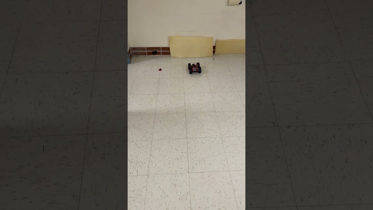
The video for the car’s motion:

The ToF raw data and the distance readings with Kalman Filter prediction:

If we zoom in, we can easily find that the prediction line relied more on the model instead of the real measurement:

The distance error from the target distance vs time image:

Second, I tested the KF with ($\sigma_1$, $\sigma_2$, $\sigma_3$) = (2, 1, 0.02), which indicated that we trust less on our model and more on the measurement.

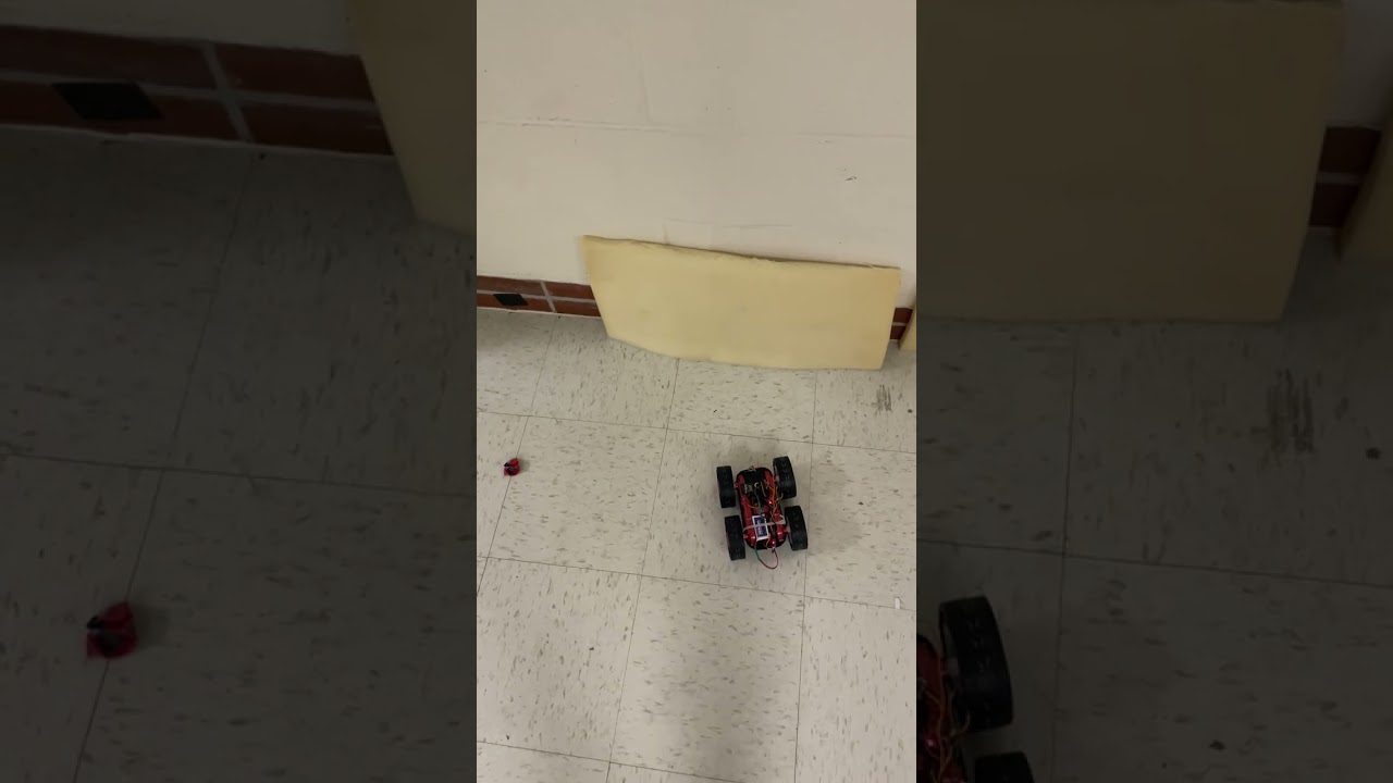
The video for the car’s motion:

The ToF raw data and the distance readings with Kalman Filter prediction:

If we zoom in, we can easily find that the prediction line relied more on the measurement instead of the model. The prediction line is nearly the same as the measurement line:

The distance error from the target distance vs time image:

Finally, I hope to optimize the KF parameters’ values to fit the robot car’s motion. After trials, I set the KF with ($\sigma_1$, $\sigma_2$, $\sigma_3$) = (0.05, 0.1, 0.2), which indicated that we trust a little bit more on our model and a little bit less on the measurement, because we indeed need the KF to predict the ToF data.

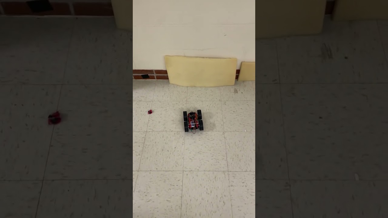
The video for the car’s motion:

The ToF raw data and the distance readings with Kalman Filter prediction:

If we zoom in, we can easily find that the prediction made a quite good job:

The distance error from the target distance vs time image:

Generally, the Kalman Filter can work similarly to the linear extrapolation implemented in Lab5. But during tests, the KF can function smoother and stabler. The lab tasks all completed!