Lab9 - Mapping
Published:
Objective
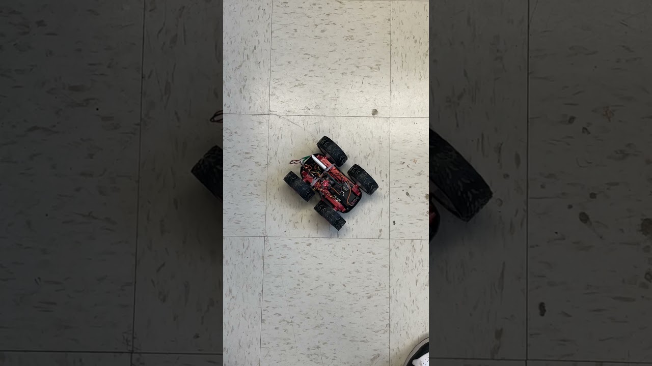
The purpose of this lab is to map out a static room; this map will be used in later localization and navigation tasks. To build the map, place your robot in a couple of marked up locations around the lab, and have it spin around its axis while collecting ToF readings.
Keyword
Mapping, Transformation Matrix
Lab Tasks
Task 1 - Orientation Control
For this mapping task, to realise the continuous rotation by a fixed angle, I implemented PID orientation controller to allow my robot car to do on-axis turns in small and accurate increments.
Here, I set the increment as 20 degrees and the car should make the rotation for 18 times within a complete cycle.
To prevent the reading drift of the gyroscope, I reset the integration term for computing the yaw from the gyroscope every time after the car reached the 20 degrees. Also, to avoid the TOF reporting false outputs if the distance to the object changes too drastically during a reading, I let the TOF record the reading after the car reached the setpoint and stayed still. Below is the related code:

I finetuned the PID controller parameters (Kp=3, Ki=0.01, Kd=0.2). This is the video for the car’s continuous rotation:
I recorded the real-time yaw readings, and make a comparison between the standard setpoint angles and the yaws:

where the first column is the index of the setpoint, the second column is the standard setpoint angle, and the third column is the real yaw reading. Basically, from the above table, the precision of the car’s rotation was quite good.
Task 2 - Read out Distances
The lab mapping court is shown as follows:

where I labeled 1~5 for each point, and the third point is the origin for the global coordinates.
To greatly decrease the error from distance readings, I only used the front TOF and got the measurements by rotating the car twice and getting two groups of data from TOF1.
For each of the point, I got the polar plot and the 2D plot for comparison. As for the transformation between these two formats, I applied a tiny transformation matrix which solved the translation and rotation. Below is the code:
For my (angle, DistanceReading) data, I pre-processed them as:

Then, they would all be transformed by the function translation as:

where dx and dy coorespond to the distance between the detecting point and the origin.
So, after transformation, the polar image and the 2D image for each point as:
Point 1 -> (0, 3):


Point 2 -> (5, 3):


Point 3 -> (0, 0):


Point 4 -> (-3, -2):


Point 5 -> (5, -3):


Generally, despite some noise, the measurements matched up with my expectation.
Task 3 - Merge and Plot
Based on task2, I merged the plot by simply “adding” all the 2D images together and got the final mapping court image:

According to this image, I can guess and highlight the wall and the objects manually as:
