Frontier-based Autonomous Exploration for UGV

This is a collection of “Frontier-based Autonomous Exploration for UGV” projects for the course ELEC4260 (Intelligent Robots and Embodied AI) @ HKUST, 2025 Spring.

Project Overview

Implemented LiDAR-based SLAM with ICP alignment, A* path planning, Bezier-curve trajectory generation, and PID control to achieve frontier-based autonomous UGV navigation and exploration.

Odometry, Mapping and ICP

March 2025 · Code

I implemented keyboard teleoperation, wheel odometry from encoder measurements, occupancy-grid mapping from 2D LiDAR data, and ICP-based LiDAR odometry for a TurtleBot.

Wheel Odometry

Preliminaries

Key steps involved in the odometry computation:

Compute the change in wheel position (incremental movement) using encoder values.
Convert the angular displacement into linear displacement (derived from the differential-drive kinematics):
- Linear displacement ($\Delta s$) is the average of both wheel displacements, which represents the robot’s forward movement:
  \[\Delta s = \frac{d_{\text{right}} + d_{\text{left}}}{2}\]
- Angular displacement ($\Delta \theta$) is computed using the wheelbase $b$ and the difference in the two wheel displacements:
  \[\Delta \theta = \frac{d_{\text{right}} - d_{\text{left}}}{b}\]
Calculate the robot’s motion in terms of position ($x$, $y$) and orientation ($\theta$):
- New x-position: $x_{t+1} = x_t + \Delta s \cos\left(\theta + \frac{\Delta \theta}{2}\right)$
- New y-position: $y_{t+1} = y_t + \Delta s \sin\left(\theta + \frac{\Delta \theta}{2}\right)$
- New orientation: $\theta_{t+1} = \theta_t + \Delta \theta$
Publish the updated path and odometry information

Implementation Details

First, the increments and displacements of the two wheels are calculated. Then, we can get the linear distance and the rotation angle of the robot movement so that we can update the global poses accordingly.
After we get the updated x, y, and theta, we can publish the updated path and the wheel odometry instances.

RViz & Gazebo Simulation

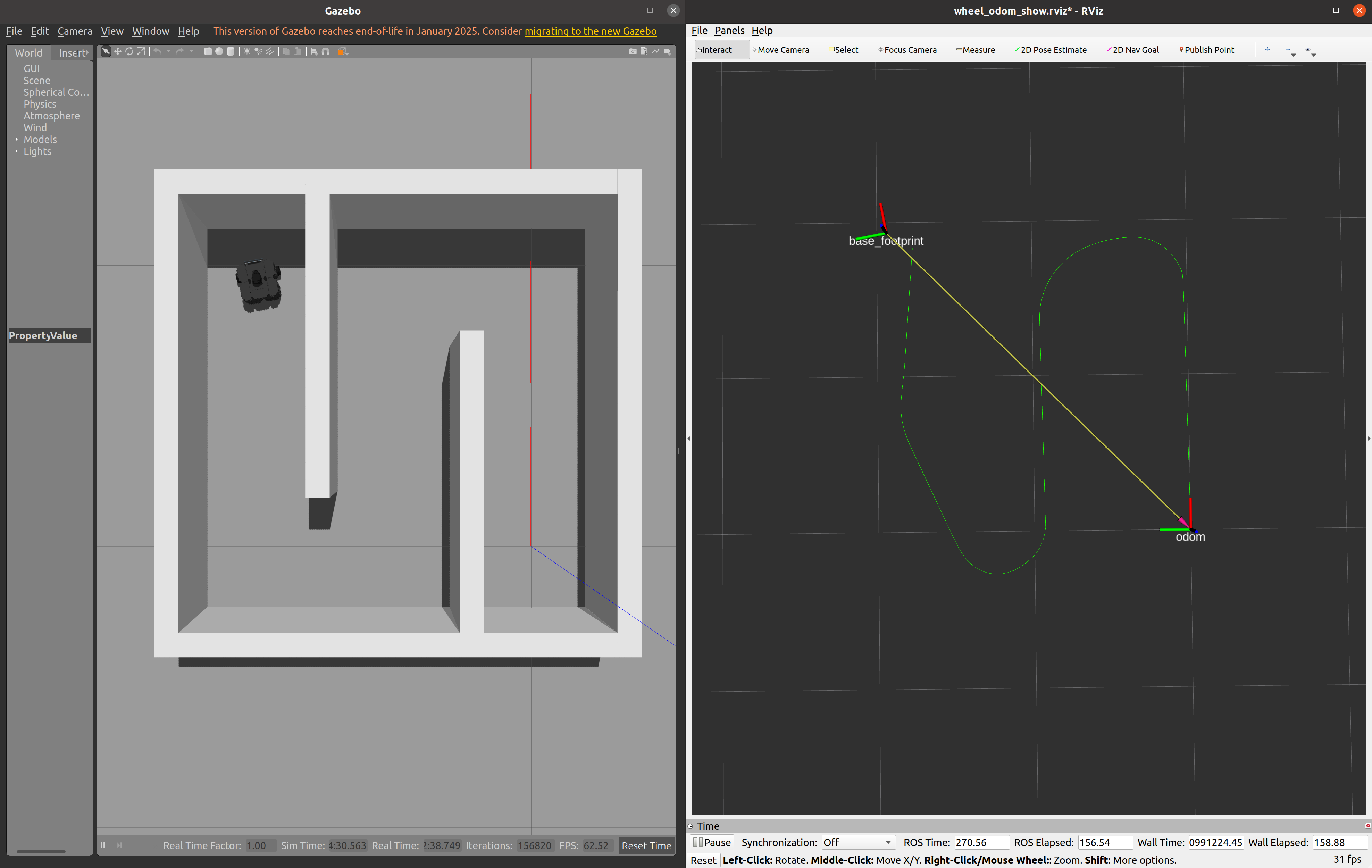
Real-World Deployment

Note: The real-world deployment is not shown in this video, considering the robot deployment can be reflected in the ICP odometry case. The following video shows the real-time RViz visualization of the robot odometry.

Occupancy Grid Mapping

Preliminaries

Key steps:

Traverse all laser measurements
Set the range threshold
Get the start point and end point
Using BresenhamLine to check the status of each grid
Publish the occupancy grid map

Implementation Details

In the scanCallback function, we determine the obstacles or the visit-or-not status of points by traversing all points from laser measurements.
At the beginning, we first determine whether the detected point is a valid point by comparing the distance with our pre-defined threshold. Then, laser-scanned points are mapped into world coordinates and converted into map coordinates. Based on Bresenham’s line algorithm, we can get a series of possible points that are scanned by lasers. We then traverse these points and determine whether a certain point is the ending point on the laser path, whose location will be labeled as an obstacle. SCAN_THRESHOLD is used to guarantee the reliability of the obstacle point. DECAY_FACTOR is used to reduce the skepticism of a certain point that might be determined as an obstacle.
After we finish updating the points based on the laser measurements, we publish the map by setting each grid’s data value to 100, -1, or 0.

RViz & Gazebo Simulation

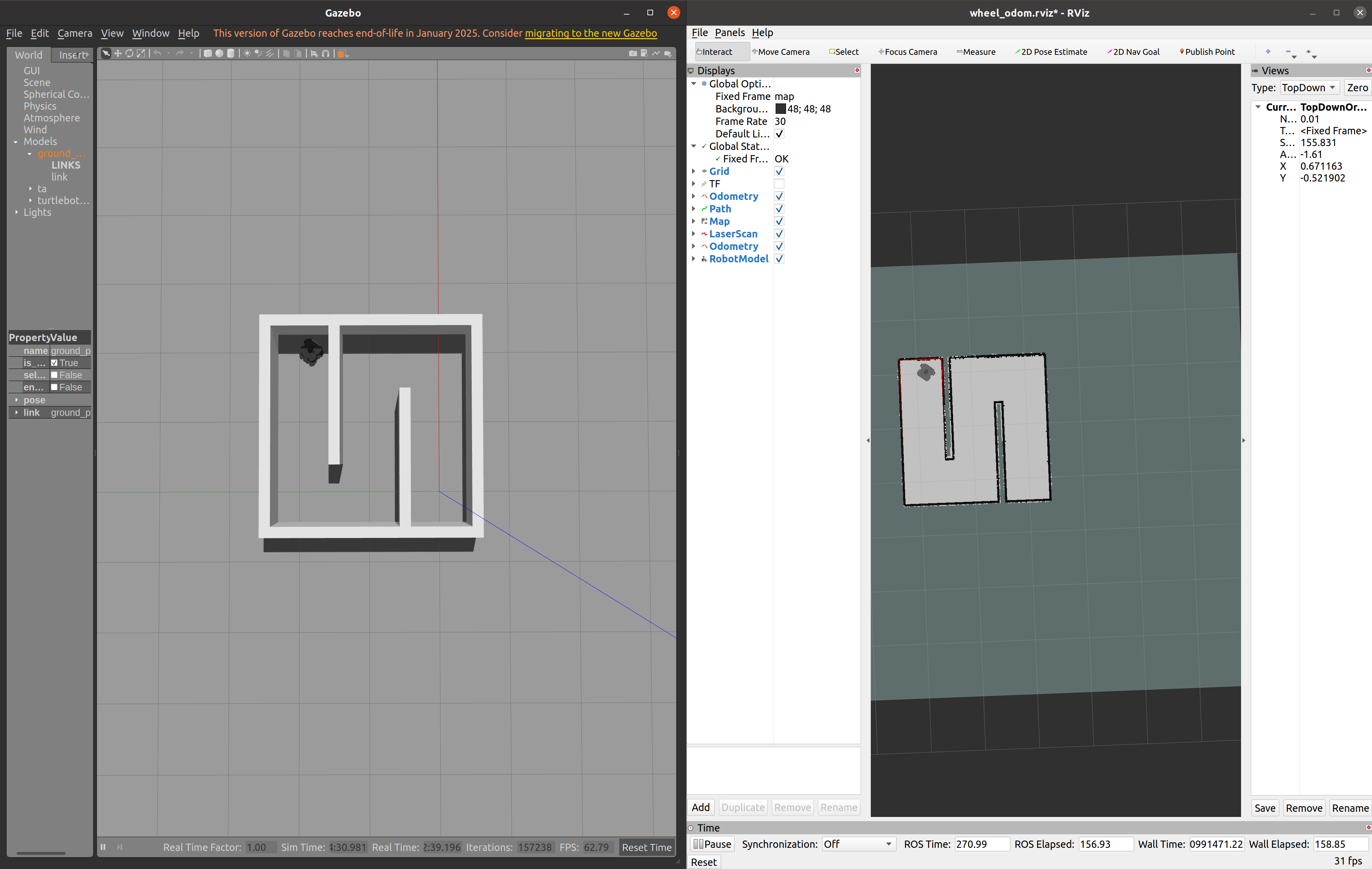
Real-World Deployment

This part is integrated with the ICP odometry case.

ICP Odometry

Preliminaries

Key steps:

Receives a 2D occupancy grid map (/map topic).
Converts the map into a point cloud representation.
Processes incoming LiDAR scans (/scan topic) and projects them into the map frame.
Uses ICP to align the LiDAR scan with the map and estimate the robot’s pose transformation (dx, dy, dyaw).
Updates the robot’s global pose (map → base_footprint transform).
Publishes ICP-based odometry (/icp_odom topic) for further use in SLAM or navigation.

Implementation Details

First, the computeBestRigidTransform2D function is finished mainly by implementing SVD for the source and target points. In this function, when $R$ is calculated by $R=VU^T$, another if statement is added to guarantee that the rotation matrix $R$ is not a flipping matrix whose determinant is -1.
As for the performICP function, we traverse all source points and calculate the distance between each source point and each target point, where we aim to find out the point pair with the minimum distance. A threshold is added to determine whether this is a valid matched point pair. Once found, the source and target points are pushed into the point lists. Such a process will be looped for maxIterations times until the convergence is reached (when the changes of x, y, and yaw are small enough).
Once we finish the ICP, we publish the odometry in publishIcpOdom. Here, we put the strong belief that the uncertainties are small. Therefore, all the variances related to x, y, and yaw are set to 0.01 in the pose and twist covariance matrices.
In the main function, the frequency of the subscriber map_sub is increased to 10 Hz from 1 Hz, which can improve the results of ICP odometry (especially the simulation updating speed).

RViz & Gazebo Simulation

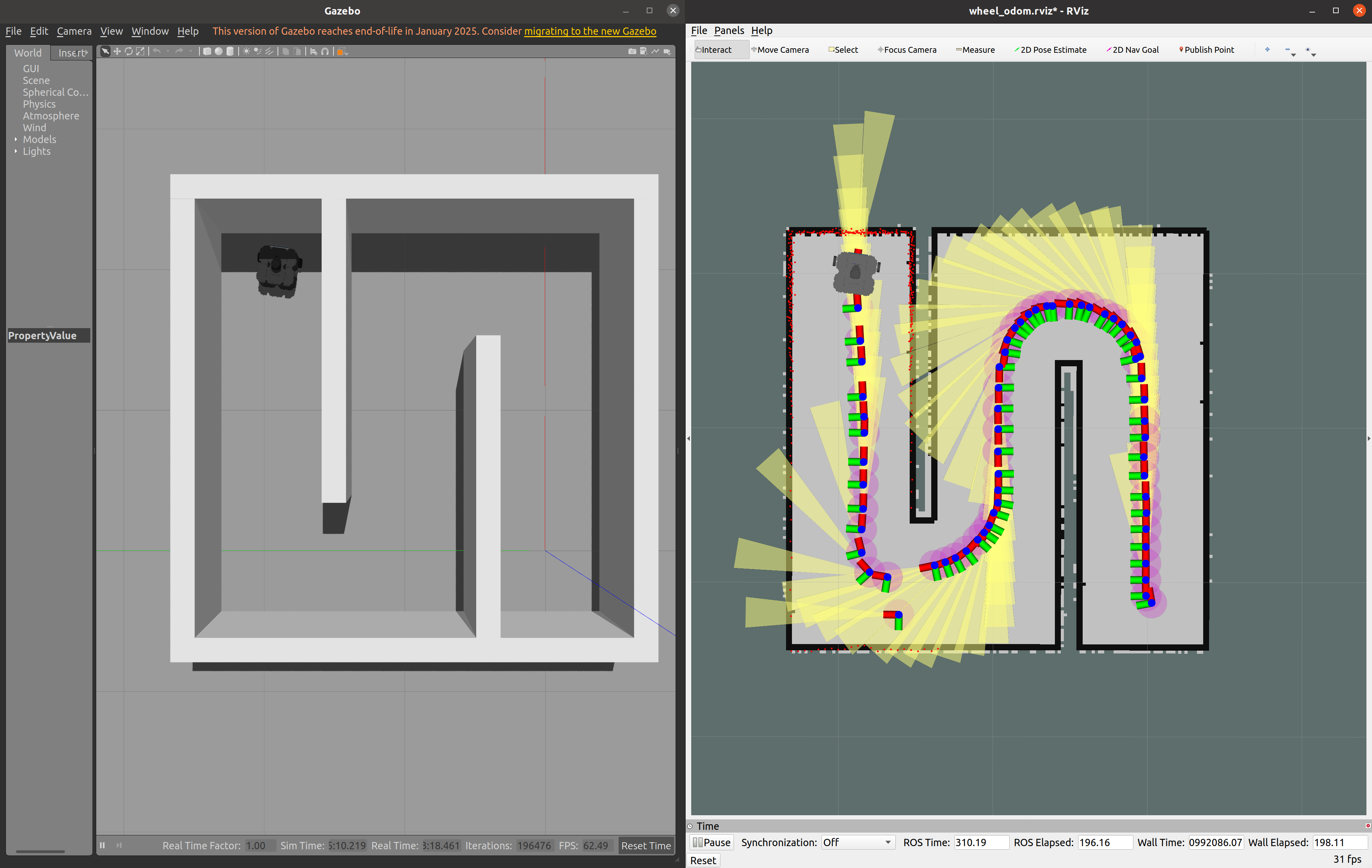
Real-World Deployment

In this video, both the simulation visualization and the real-world deployment are shown simultaneously (picture-in-picture).

Path Planning, Control and Exploration

March 2025 · Code

I implemented A* path planning with obstacle inflation and Bezier-curve smoothing, PID-based path tracking, and frontier-based exploration in unknown environments.

A* Path Planning

Key steps involved in the A* path planning:

Use the Bezier curve to effectively create smooth paths.
Inflate the obstacles with a certain radius to ensure the robot can avoid them.
Use the A* algorithm to find the shortest path in the inflated map.

Bezier Curve

Defined by a set of control points, the Bezier curve smoothly interpolates between these points. Their use in trajectory planning offers the following benefits:

Smoothness of Path
Guarantee of End-Point Convergence
Applicability to Various Types of Path Planning

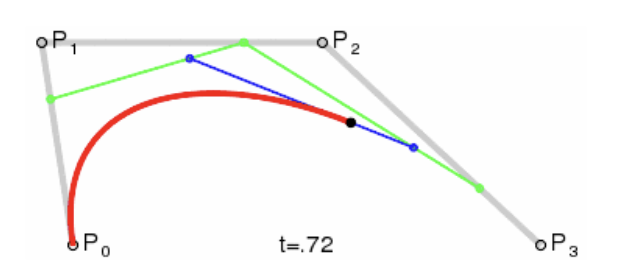
For a cubic Bezier curve, which is the most commonly used in trajectory planning, the curve is defined by four control points: $P_0$, $P_1$, $P_2$, $P_3$.

The cubic Bezier curve formula is:

\[B(t) = (1-t)^3P_0 + 3(1-t)^2tP_1 + 3(1-t)t^2P_2 + t^3P_3, \quad t \in [0, 1]\]

where: $P_0$ is the starting point, $P_3$ is the ending point, and $P_1$ and $P_2$ are the intermediate control points that determine the shape of the curve. The general case of a Bezier curve is shown as the following figure:

Inflation Radius

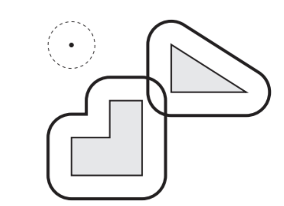
By expanding the radius of the obstacles, we can create a “safety buffer zone” for robots. Here, we first convert the robot radius into grid cells by $inflated\ cells = \frac{robot\ radius}{grid\ resolution}$. Then, iterate through each cell in the occupancy grid and find obstacle cells. We then expand each obstacle cell by the inflation radius in all directions and make sure to check the boundary of the grid.

A* Algorithm

A* is a popular pathfinding algorithm that efficiently finds the shortest path in a weighted graph. It combines the advantages of Dijkstra’s algorithm (guarantees the shortest path) and greedy best-first search (efficient pathfinding).

Key Components of the A* Algorithm:

Cost Function
The total cost $ f(n) $ of a node $ n $ is calculated as:
\[f(n) = g(n) + h(n)\]
where:
- $ g(n) $: The actual cost from the start node to the current node $ n $.
- $ h(n) $: The heuristic estimate of the cost from the current node $ n $ to the goal node.
Heuristic Function ($h(n)$)
$h(n)$ should be admissible, meaning it should never overestimate the true cost to reach the goal. Common heuristics include:
- Manhattan Distance:
  $h(n) = |x_2 - x_1| + |y_2 - y_1|$ (for grid-based movement with 4 directions).
- Euclidean Distance:
  $h(n) = \sqrt{(x_2 - x_1)^2 + (y_2 - y_1)^2}$ (for continuous or diagonal movement).
Priority & Visited Queue
- Priority Queue (Open Set): A priority queue containing nodes that are candidates for expansion, sorted by their $f(n)$ values.
- Visited Set (Closed Set): A set of nodes that have already been expanded to avoid revisiting them.

A* Algorithm Steps:

Maintain a priority queue to store all the nodes to be visited
The heuristic function $h(n)$ for all nodes are pre-defined
The priority queue is initialized with the start state $X_S$
Assign $g(X_S)=0$, and $g(n)=\infty$ for all other nodes in the graph
Loop
- If the queue is empty, return FALSE; break;
- Remove the node $n$ with the lowest $f(n)=g(n)+h(n)$ from the priority queue
- Mark node $n$ as visited
- If the node $n$ is the goal state, return TRUE; break;
- For all unvisited neighbors $m$ of $n$:
  - If $g(m)=\infty$:
    - Push node $m$ into the queue
  - If $g(m)>g(n)+c(n,m)$:
    - $g(m)=g(n)+c(n,m)$
- End
End loop

Implementation Notes

Angle difference calculation → I choose to approximate the angles for p0 and p3 using their adjacent points, which is angle_diff = abs(calculateAngle(p0, p1) - calculateAngle(p2, p3)).
Interpolation number → The number should not be too big or too small. If it is too big, the Bezier curve will be too smooth. Although the module for detecting inflated obstacles is continuously working, very smooth curves will impact the computational efficiency. If the number is too small, then the curve will be zigzag, which will bring challenges to the controller. In the code, this number will be the bigger one between the least number 5 and the numerical result of the scaled angle difference value. The robot’s actual speed limit and the sampling number of the raw curve determine that the interpolation number will not be too big.

RViz Simulation

PID Control & Path Following

Preliminaries

The three components of PID control are:

Proportional (P): The proportional term produces an output that is directly proportional to the current error. It aims to reduce the error by applying a correction proportional to the magnitude of the error.
Integral (I): The integral term accumulates past errors over time, aiming to eliminate residual steady-state error that may be caused by system biases.
Derivative (D): The derivative term predicts future errors based on the rate of change of the error, helping to dampen oscillations and improve system stability.

The PID control formula is:

\[u(t) = K_p e(t) + K_i \int_0^t e(\tau) d\tau + K_d \frac{de(t)}{dt}\]

Ziegler-Nichols Method is applied to tune the PID parameters.

Implementation Notes

To make the tuning fast and convenient, I put the PID gain parameters into a testing launch file (no need to type rosrun one by one manually) and also disabled Gazebo’s GUI (save time for shutting down and restarting the GUI). In this way, I can restart and initialize the map status in the RViz and use the rosparam set command to finetune the parameters dynamically. The private_nh and the method of initializing the gain values should be adjusted accordingly. For example, the kp_heading should be initialized using private_nh.getParam("kp_heading", kp_heading_), instead of using private_nh.param(xxx). After implementing A* path planning and with the raw skeleton of the frontier explore code, I finished finetuning the parameters roughly to guarantee the controller can basically work.
With the implemented A* script, I disabled all the commands related to the “Robot Stop” in the PID controller source file, which can greatly reflect the performance of the controller when the robot is getting closer to its steady state. Also, I increased the max linear/orientation speed limits to ensure the performance of the controller was not masked by the robot’s slow speed. Typically, the goal_distance_tolerance is decreased to 0.05 from default 0.2, which is just to test the linear distance controller. (There is no point in finetuning the PID controller if the frontier exploration, which will update the inflated grids, is not implemented. So, I can just try my best to optimize the distance controller.)
Currently, the robot’s absolute max speed is not that high. Therefore, I only use the PD controller without the I-term to maximize stability. The optimized PD controller performs quite well under a reasonable max speed limit (higher than the default limit). The tuning process was conducted using the Ziegler-Nichols Method.

RViz Simulation

Frontier Exploration

Preliminaries

Frontier points are identified as the boundary points between explored and unexplored regions. These are locations where the robot can make progress by exploring new, previously unknown space.A frontier point is defined as a free space (value 0 in the grid) that is adjacent to an unknown area (denoted by -1), while the robot has direct access to this free space.

This frontier exploration task processes occupancy maps, inflates obstacles, and detects frontiers for autonomous exploration. When the robot reaches a goal, it triggers the next frontier selection.

Implementation Notes

The general steps of the frontier exploration are:

Build inflated obstacle: Refer the A* part. When selecting the forward point, it is necessary to avoid choosing a location within the inflated radius area to prevent the robot from colliding with obstacles.
Frontier Detection:
- Iterate over every cell in the occupancy grid.
- Identify frontier cells: A frontier is a free cell (0) adjacent to an unknown cell (-1).
- Store valid frontier coordinates in frontiers.
Frontier Clustering:
- Traverse each frontier point.
- Create a queue, add the current frontier point to the queue, and mark it as clustered.
- Remove a point from the queue and expand to its neighbors.
- If a neighbor is an unclustered frontier point and reachable, add it to the queue.
Find the largest cluster: To select the largest cluster from a given list of frontier clusters. A cluster is a group of adjacent frontier points (unexplored boundaries of the known map). The function determines which cluster has the most points and returns its index.
- Initialize tracking variables
- Iterate through all clusters
- Compare cluster sizes
- Return the index of the largest cluster

Something to note while implementing:

When the frontier points are getting clustered, we should use push_back or emplace_back to push the current cluster into the cluster list clusters, though there is no significant difference between these two commands. They both copy value-by-value, which cluster will not be empty at the end of each loop. If we use std::move to push the cluster, it will move the cluster itself without copying, which will make the cluster empty at the end of each loop. This will prevent adjacent clusters from forming an integrated larger cluster.

RViz Simulation

Real-World Deployment

With all the components implemented, the deployment on the Turtlebot3 is done to test the performance, which is shown as the following video (both the simulation visualization and the real-world deployment are shown simultaneously):